Asset-Allocation Showdown

Author: Marco Santanche

Last month, we discussed asset allocation and its crucial role in our portfolio’s performance. Many traders, especially non-professionals, believe that any strategy, including technical analysis and fundamentals, can be applied to assets individually. But this clearly results in misjudging the impact of the asset-allocation problem - that is, the problem of how much of the capital should be assigned to each of their separate strategies.

While many years have passed since Markowitz Portfolio Optimization (Mean Variance Optimization) and the birth of Modern Portfolio Theory, and the world of asset allocation has progressed towards even more sophisticated methods, it is not uncommon to see naive or simple asset-allocation methodologies.

We will now measure the impact of such asset-allocation methods, and we will observe what advantages and disadvantages they bring.

Naive: equal weights

The simplest, yet very misunderstood, asset-allocation system is the equal weighted portfolio, also called 1/N or naive asset-allocation system.

It is very intuitive, and it appears to be a very good idea at the beginning. This asset-allocation system allocates the same portion of capital to all assets, regardless of their prices, risks and potential future developments.

The intuition is that, while we cannot predict the future, we can still control our capital, and allocate equivalent portions of our portfolio to all the available assets.

The advantage of such an approach is that we have the (wrong) feeling of keeping all risks under control. Imagine a trader who has a powerful trading strategy on securities separately, some magical tools that allow them to guess 60% of the bets on one asset. Now, if they had to allocate their money, they would probably invest equally in all instruments.

It is not uncommon to think this way. But the problem is, the control we have over the strategy is only an illusion, for multiple reasons.

First of all, we are not really making any assumptions. We are indeed assuming that all assets have similar risks in our portfolio, and the gains (and losses!) are equivalently large for any asset class, regardless of that being an equity index, a fixed-income security or an option. This clearly increases our risk dramatically, because it is much more likely that an option will lose 40-50% of its value (even 100%) when compared to the same event on a fixed-income security. This definitely increases returns, but, even in case of a very positive backtest, we should beware this solution as it is often not only unreasonable and risky, but also unrealistic.

The most important reason why that is the case is the timing: we are assuming nothing about the correlations of our system and securities, which will eventually hit for sure, because we are investing in multiple assets, regardless of what we think we separated. If the equity strategy falls 2% and the fixed income earns 1%, we are not profiting, even if the proportion between positive and negative trades remains constant.

But probably the most important issue is timing with regards to rebalancing: when should we start our equal-weights investment? How often should we rebalance? Should we let our weights drift dramatically from the initial investment? A lot of answers that we need for practical implementations, and that lead us to think that, no matter how good, the results obtained from tests or simulations using equal weights would make no sense for our portfolio.

Proportional weights

In some cases, and factor investing is one famous example, investors or portfolio managers allocate capital according to the signal they are analyzing/using. In investment management and trading, a signal is a methodological approach that gives us the direction, intensity and time at which we should invest in a single security, or in a basket of securities.

Trading signals are important, because they can give us an edge in active investment management. Some very simple signals, based on factors such as momentum, can provide us with superior performance when compared to buy and hold. The time at which we observe them can be scheduled based on specific dates, events, or both.

In factor investing, we consider for example factors such as momentum, value, dividends etc. Any of those can be a signal, suggesting that a security would be profitable if overweight/purchased or even shorted. Nothing prevents us from underweighting securities, or having exit signals, based on the same methodology.
And many portfolio managers and professional investors started allocating their capital according to the signal. There are multiple ways of proceeding: one could rank the securities and allocate according to their ranking, or base it purely on the signal (eg., a signal of 0.5 and another one of 0.25 would result in ⅔ of the portfolio in the previous and ⅓ in the latter).

While this is a reasonable approach that takes into consideration some forecasting model or method, there are also some very considerable risks: for example, there is no link between the signal and the probability that it would be wrong. And while a large signal would rationally lead to a higher asset allocation, we can’t just ignore the possibility that our signal is under- or overestimated, especially when we are basing our allocation on the same. It would result in a double error, in case the signal is not only wrong in its timing or direction, but also leading to a larger allocation. And the impact might be crucial even if the “true” signal would lead us to rank the security lower or higher than what the “false” signal tells us, and we base our portfolio construction on this wrong ranking.

Modern portfolio theory

We need to consider a more scientific approach for this simple showdown. Markowitz and his portfolio optimization has been ruling the academic courses for ages, and with good reason, being a necessary contestant in this episode.

His model is simply better than both our contestants, at least on paper. The methodology and assumptions make more sense, since we can use this powerful tool not only to allocate according to our signal, as defined by the proportional weighting method, but also by clearly defining what risk is, and how to reduce it.

Such a model is - ideally - the target for all investors: we should take into consideration both aspects, returns and risk, and in some cases some additional factors, such as skewness, kurtosis, transaction costs, etc. But at the time (1952), the model suggested by Nobel Prize winner Harry Markowitz was definitely what we needed.

What are the major concerns? There are multiple disadvantages, some of them arguably still hard to manage with other models today. The portfolio-optimization routine is, for example, very sensitive to estimates and potential errors in the signal; the rebalancing problem remains, because there is no clarification on how often we should adjust our portfolio; and so on.

Risk parity

Many are aware of the term “risk parity”, but not many know how subtle the differences in implementation can be.

Very often, a risk-parity approach is compared to the individual volatilities of asset returns. According to this implementation, the proportion of capital is identified in a similar way to what one would do in the signal-oriented allocation - by giving a weight which is inversely proportional to the volatility of every single asset compared to the other assets’ volatility. For example, if an asset has a volatility of 2% and another one exhibits a 4% volatility over the same period, this method would invest 50% in the first asset and 25% in the second asset.

This clearly ignores correlations. Such approaches should be avoided at source, because not only there is a big risk of underestimating the impact of correlations (both assets could go negative at the same time, and our portfolio would not be saved by our allocation), but also, volatility is often considered a wrong metric for risk (although widely used, thanks to Markowitz).

The best implementation of risk parity is the equal-risk-contribution approach. When we consider correlations, the actual target of risk parity becomes to equalize the contribution of each asset to our portfolio’s volatility, which is not only defined by the individual oscillations around the mean, but also the co-movements of such oscillations.

This is possible with optimization routines and a solid mathematical approach. The disadvantage is that we are - again - forgetting about potential signals or rewards. But many practitioners argue that asset allocation and portfolio management are actually much more oriented towards risk than returns.

Experiment definition

We will now consider a portfolio-construction process for the period January 1 2015 up to November 1 2023. We might use prior data to fit the models, depending on the case. The minimum timeframe will be one day, and we will rebalance monthly for all of them.

For all of our models, we will use momentum as a trading signal, defined as the change in closing price over a 22-day timeframe (proxy for one month). This will lead to the possibility of short selling securities, if their momentum is negative. In all cases, the portfolio will be fully invested.

The universe of ETFs in analysis are as in Table 1:

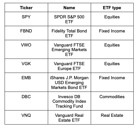
We are particularly interested in seeing the difference in results depending on the different times in the market.

The models in analysis will be:

• Equal weights. We will rebalance monthly, without additional criteria. The sign will change according to our signal.
• Proportional weights. This model will give a weight to each asset according to their momentum over the one-month horizon. The weight will be determined by the value of the return over this period divided by the absolute sum of values.
• Ranking weights. In this case, compared to Proportional Weights, we will assign our weights according to the ranking over the total, in absolute terms. The sign will again be determined by the signal.
• Mean-Variance Optimization (MVO, Markowitz). This model will determine the expected returns based on the signal, and allocate according to the famous Mean-Variance Optimization process.
• Risk parity. In this case, the contribution to volatility might change according to the sign of the investment. Thus, we will use our trading signal to determine the direction that we are going to trade, and the covariance matrix will be adjusted according to our intention to buy or short.

Results

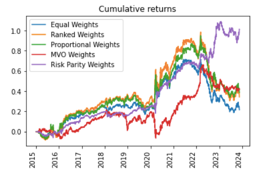
Let us have a look at the performance of the different allocation models in this simple example.

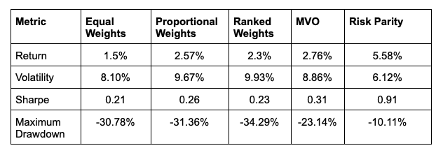
And some performance metrics in the table below, referring to the aforementioned period. Return, risk and Sharpe Ratio are annualized figures.

Key intuition

The simplicity of these models still outperforms Markowitz dramatically, especially in risky times. When the market moves sharply down, which normally coincides with bad estimates from our signal (Momentum), the covariance matrix doesn’t really help in diversifying our portfolio as per the Mean-Variance Optimization.

We have already discussed how simple the model is, yet more sound than the basic methodologies; still, if the performance is so dramatically volatile, this explains why current providers do not use it in live portfolios, but prefer some less sound and more stable approaches (in terms of performance). However, we also have to recognize that the Mean-Variance Optimization not only eventually outperforms (in terms of returns and risk) almost all other alternatives, but it also generates a better Sharpe Ratio and a much lower drawdown.

The three “dummy” alternatives (Equal Weights, Proportional Weights, Ranked Weights) are not sufficient. The first one is the worst of all in terms of Sharpe Ratio, slightly worse than Ranked Weights (although the Maximum Drawdown is slightly better). But generally speaking, none of these strategies is capable of turning our signal into a winning one (although we are also aware that the signal is a very basic one used for comparison, rather than alpha generation).

But let us now come to the winner: Risk Parity is superior in all terms. Although it underperforms the three dummies for a long period of time, it eventually comes out as a winner in 2023, where its fundamental difference in allocating to the riskier assets turns a losing signal into a winning one. It appears that 2022 is the year of the crash for all the three simple allocation models, and the rebound for Risk Parity and Markowitz, which continue their outperformance in 2023 (it sounds like it is linked to inflation, on a side note).

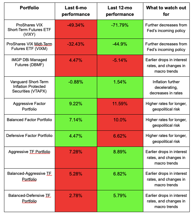
Update on strategies

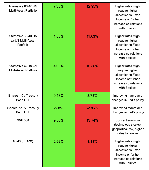
The past six months have been positive for almost all portfolios and ETFs, excluding trend following (DBMF is also a trend-following strategy) and volatility. Over a single year, however, the picture is mostly negative, with exceptions made for volatility, short-term TIPS, short-term bonds and our custom trend-following strategies.

Updates as of November 16:

Trading strategy is based on the author's views and analysis as of the date of first publication. From time to time the author's views may change due to new information or evolving market conditions. Any major updates to the author's views will be published separately in the author's weekly commentary or a new deep dive.

This content is for educational purposes only and is NOT financial advice. Before acting on any information you must consult with your financial advisor.