How Trading Signals Can Enhance Investment Strategy
Author: Marco Santanche
Although asset allocation remains crucial in our investment process, some of the most active retail investors might want to trade with an edge. This is where signals become important: most of the data out there can be used as a signal, such as technical analysis, macroeconomic variables, and orderbook data.
But the main advantage to using trading signals is the discovery of alpha: the true added value that active strategies seek in their setup.
Alpha is given by a combination of factors, including trading signals and asset allocation. With a positive alpha, we do not have the guarantee of a good strategy though: first of all, we must consider its net value, which includes fees, spreads and slippage; secondly, a high alpha investment might still have a high beta, such that the risk might become unbearable, or even negative beta, which leads to underperformance during rallies in the benchmark.
Can we achieve outperformance when using trading signals? This initial question is often overlooked by many retail investors (and sometimes even institutional ones). But what we need to address first is: does our signal make sense?
How to obtain trading signals
A trading signal can be generated by any sort of data. If we consider an MACD indicator, for example, we might go long if one of the two moving averages moves above the other one, and short otherwise. Of course, rules can change, and for example this can be applied to long-only strategies by exiting the market instead of going short.
Many datasets, including the widely available open-high-low-close-volume data (OHLCV), allow us to calculate some indicator or signal to enter into a position. But with the data revolution happening in recent years, institutional investors are looking for much more sophisticated datasets, which can allow them to outperform peers by accessing unique information, such as insider transactions, earnings forecasts or announcements, web traffic, meteorological data, etc.
What truly matters is the way we process the data. Even if just using OHLCV datasets, there might be some information lying under the surface that we can access with statistical calculations and adjustments; a simple example is momentum trading, which just uses past returns to identify a universe of assets to invest in. We then need an asset-allocation stage that allows us to expose ourselves to these factors in the proper way.
But before trading or backtesting, it would be useful to assess the meaning of a signal, why it matters, why it should work, but most importantly: if it works.
How to test a signal before using it
It is always difficult to research strategies in finance: it is very easy to see what does not work, but anything that works seems fishy.
A backtest is not the right tool to check if a signal works. Unfortunately, many still think that running thousands of backtests and selecting the top-performing one is the process followed by most professionals and institutional investors.
Why is this wrong? Because a backtest will work, at some point. Coincidentally or not, but we will not be able to guess if it is due to the randomness of guessing or actual solidity of the strategy. And especially when using different combinations of parameters (with the MACD example above, it might be something like testing all lags from 1 to 10 for one of the two moving averages, and from 20 to 50 for the other one), selecting the optimal one according to the backtest is a recipe for disaster. In fact, there is no actual rationale behind the selection of those numbers, it is just what overfits past data, with no implication for the future. And, especially when testing for sensitive datasets (imagine a stock with specific business cycles, mergers or acquisitions, product launches etc, or even macro events such as the Covid-19 pandemic, inflationary regimes, etc.), this becomes very dangerous.
Even if we run a single backtest, we need to take into account the 'luck' factor: how many trades were successful, when were they successful (are they all close in time or consistent) and how much do we make with winning vs. losing trades?
In summary, even if the backtest gives a positive return and Sharpe Ratio, we need evidence that the strategy works.
Before backtesting, and only in sample data, we need to assess if the signal makes some sense. The problem is, if we split our data historically, the signal might work in the past, but it might not work in the future (Type I error, or false positive, in statistics) or the signal might work in the future but not in the past (Type II error, or false negative). While the previous leads to financial loss, the latter might lead to opportunity costs.
How can we address this issue and avoid both errors to the best of our capabilities? Most importantly, how can we ensure we identify consistently working signals?
There are two main paths:
- Mathematical Optimization. Some problems, especially in strategies like time series modelling or statistical arbitrage, might have an analytical solution that can be found with a specific formula or optimization routine.
- Synthetic Data. If we build large datasets of random data, similar to the one we are going to test, we might be able to avoid overfitting.
A possible third path, suggested by Graham Giller, is to select a different asset and test our alpha on it. The basic assumption is that if we select an asset with low correlations with the original one, our strategy might work for the actual target one. The low correlation implies that future performance might differ greatly from the past one, so the training set is somehow not predictive of future returns.
We will focus for the moment on the methodology to identify meaningful signals. Method 1) might not need a grid search algorithm, since it would have an analytical solution for the best parameters in our model, but it is often unfeasible or very complicated for retail investors, and it does not apply to all signals. Both methods 2) and 3), plus the (suboptimal) option of testing on past data, are suitable for signal testing on any setup. Additionally, we are not targeting the optimal selection of signal parameters, but rather the significance of any signal, with any set of parameters, found in any possible way, optimized or randomly selected.
Statistical methods
It is not uncommon to hear about the Mean Squared Error (MSE), or Mean Absolute Error (MAE), and others. These statistical metrics help us identify the error made by a signal in forecasting its target variable. Imagine we have a predictive model based on a number of variables: the signal will eventually digest the numbers and return a prediction, which might be on return, volatility, or something else.
The error made by this estimate is normally assessed with MSE or MAE. But another way to look at it is as a classification model: we might have a +1 or -1 (positive or negative returns, for example) and use any metric relying on the confusion matrix (Precision, Accuracy, F1 Score, etc). However, the encoding in +1 and -1 is also subject to a parameterization, since models normally provide us with probabilities (of being in one or the other class), and we might be interested in 'cutting' the classification in a different way (e.g., if +1 is predicted to have a 60% probability, we might consider it too low, since we might want to be 70-80% sure that the market will move up).
Although these are robust ways of testing signals, they are not necessarily sufficient. A high or low accuracy might still lead to under- or overperformance in production, because we are not testing the ability of the signal to time the most relevant returns in the market.
Performance metrics
Yes, we can look at performance (on past, synthetic, 'correlated' datasets) to identify the importance of a signal, and if we should use it in the future. But this is not the return we get from using the signal, and the Sharpe Ratio is likely suboptimal as well.
What we need from an individual signal, especially if we use many signals together, is its relevance to identify positive or negative times in the market, which we might also summarize in two words: market timing.
Timing the market is difficult, but this must not be a barrier to test if a signal has some predictive power. It is very clear, for instance, that inflation and interest rates do drive the markets for quite some time.
To assess the performance, we can use a few statistical tests on the benchmark returns (e.g. the asset we want to invest in) and the 'strategy', which in this initial step just constitutes the returns of the benchmark times the signal (direction, if positive-negative-null, or size, if we have some number that specifies the intensity of the signal, such as the probability).
After building this “dummy” strategy, which might or might not coincide with our final application of the signal, we can measure its performance through some famous indicators, such as those summarized in the below table.
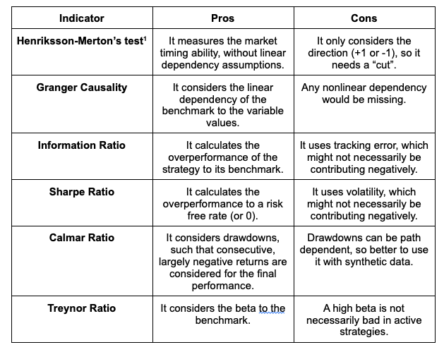
With regards to the above, the usual - still meaningful - clarification must be done: no metric is perfect. However, we should tend to prefer some over others, and in particular we are talking about the Information Ratio over the Sharpe Ratio: it does not make sense to consider the volatility of a single asset’s returns, but it makes sense to consider the distance from its benchmark, especially in this case, since we will use the signal to produce returns that come from the benchmark directly. Nevertheless, this might be more or less relevant to you, depending on your preferences. A generally upward-biased tracking error would still produce a low Information Ratio, but it would be actually wrongly penalizing the strategy/signal.
For those who do not know the Henriksson-Merton test, it is a very useful test to identify the market-timing ability of a manager. Similarly, we can deploy it with a different meaning on trading signals: if the signal has market-timing ability, we include it in our model. And this applies to the final returns of our strategy (after backtesting the fully-ready setup): in order to validate the backtest, we must look at many indicators, and the HM test is definitely one of the most important ones to consider.
A bit weaker is the case for the Granger Causality and Calmar Ratio: the previous has a linear restriction which might result in unreasonableness (imagine a signal providing exponential returns: it would not be considered as good as a linear one). But on the other hand, we must admit that using the variable directly might be more interesting than building up returns with the sign of the signal, to truly test if the variable causes (to some extent) the reaction on the benchmark. For the Calmar Ratio, the problem is the usual bias of drawdowns: if a signal does not work for some time, it might cause a large drawdown and low Calmar Ratio, but that does not mean that the signal is not effective at all, since maybe it is only from some period on, or on another synthetic sample. However, we definitely need to consider the relative size of returns and drawdowns as compared to e.g. the Information Ratio, which would penalize the high tracking error from lower-risk signals.
Experiment definition
We can now consider the performance of some signals over an in sample period, measure their performance, and see how they do out of sample. While very simplistic and ignoring asset allocation, this is the perfect way to exemplify how to test signals and check for their validity before using them.
Please bear in mind that signals might still work after our filter (negative performance/statistical metric). A number of reasons can motivate this possible mistake: randomness of future data or synthetic data, changes in the power of the signal, error in the statistical test (no test guarantees a 100% probability of being right), and so on. But again, we should distinguish between Type I Errors (false positives: a signal is deemed predictive, while it is not) and Type II Errors (false negative: a signal is deemed negative, while it is not). Type I Errors can be reduced by implementing a number of different tests. Type II Errors should also conceptually be reduced, but it depends on the selection rules (how many tests does one signal 'pass' to be selected?)
The signals we are going to consider are a couple of classic technical indicators, past returns, and inflation on the SPY and GOVT ETFs. For inflation, we are going to source the data from the Fred API; for asset prices, we will use Yahoo Finance.
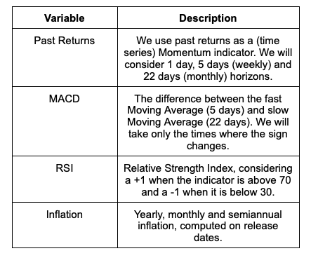
Kindly note that these signals do not only have different timeframes, but they might also have different impacts. In this sense, we will need to also measure the performance over different horizons. This is why we will consider returns for the next day, the next week and the next month for each of the variables.
The ratio in the exam will be the Calmar Ratio, in order to show how its bias can lead to bad decisions in signal processing, but also in strategy evaluation. As mentioned, it is subject to some clear limitations: the path matters, so it might be that a past path does not repeat. Moreover, it is sensitive to outliers, in the sense that a single, large return (either positive or negative) might turn the metric upside down. However, it serves the purpose of analyzing the performance of a signal over time and it somehow keeps track of the size of the signal performance by cumulating returns.
After measuring the performance over 6 years (from 2015), we will test the performance of the best signal for the two ETFs in the remaining ~2 years, for a split that resembles a 75%-25% in sample/out of sample subsetting. Although imperfect, this is a good starting point to put this methodology to work.
Results
Calmar Ratio Table
*: this variable cannot cumulate over time, because it is a constant signal. Thus, its 5-day and 22-day horizons will be equal to the 1-day horizon.
In this case, we are looking at the best predictive variable for our metric and each of the two universes. Conceptually, any signal will lose its predictive value over some time horizon; however, this might actually not be the case if the reaction to the signal accumulates over time (for something trend-settling like inflation, or maybe MACD).
Highlighted in green, we can see the (significantly) positive results. For SPY, we identified momentum as a meaningful variable for the next day, but also the MACD indicator and the RSI indicator, which seems even more powerful on the 5-day horizon contrarian sign. Inflation works best as a direct indicator over the long term (22 days), although it is counterintuitive. But we always need to keep in mind that this analysis is ignoring other possible influences on the time series, returns, and macro aggregates. Similarly, for GOVT we have inflation as a meaningful indicator (but again on the less intuitive side).
Out of sample performance
The problem with our CPI indicator is, for example, that for the 2022 horizon all values are positive, and our performance is not that interesting as it relates to the original strategy. A Calmar Ratio filtering completely ignores the comparison with the original series.
But if we examine the performance of something more dynamic, like positive momentum for SPY and negative momentum for GOVT, things become more interesting (gross of trading fees):
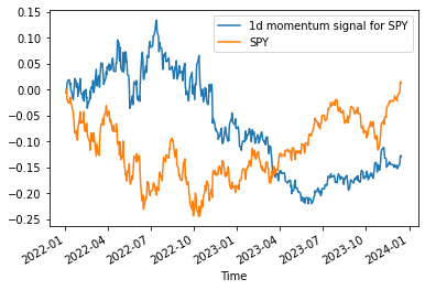
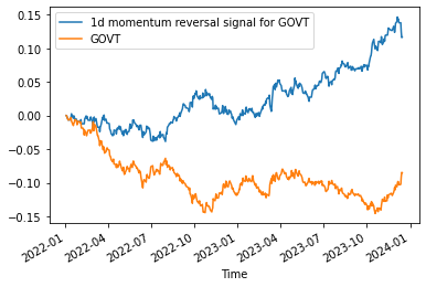
It appears that SPY’s signal is not as strong as anticipated over time, or maybe some structural change made it less effective over time (in 2022 it starts to drop in performance only after July). With regards to GOVT, it seems instead that our system is more consistent over different regimes.
Conclusion
It is definitely possible to build and use our own trading signals and select them carefully before running a backtest or strategy simulation. All indicators are imperfect, and they are not necessarily stable over time; however, a signal-processing routine before modelling or preparing an asset-allocation strategy can add considerable value to our investment.
Update on strategies
Seriously improving YTD performance for many ETFs. Volatility fell, managed futures struggled due to inflation; however, TIPS over the short term still managed to outperform. Factor investing is performing well, although underperforming the S&P 500; very nice performance from 60/40 as well, and our US variant is outperforming BIGPX.
Updates as of December 16:
Trading strategy is based on the author's views and analysis as of the date of first publication. From time to time the author's views may change due to new information or evolving market conditions. Any major updates to the author's views will be published separately in the author's weekly commentary or a new deep dive.
This content is for educational purposes only and is NOT financial advice. Before acting on any information you must consult with your financial advisor.