Factor Investing: A Comprehensive Guide

Author: Marco Santanche

1) Factor Investing: A Brief Introduction

What is factor investing?

It all started with a paper from Fama and French in 1992, where they tried to explain the outperformance of some groups of stocks compared with others using empirical, measurable factors that could be observed on the market.

The Capital Asset Pricing Model (CAPM), the most widespread model at the time and still an important one in finance, explains the returns of stocks by using just one factor (the market risk, or Beta, β). Although extremely important, this factor is not able to explain the observable differences between groups of stocks. Fama and French came up with a solution to this problem, by adding (initially) two factors: small caps and high-value stocks.

The three factors, which we will call β, SMB (small-minus-big) and HML (high-minus-low value), can be considered a fundamental change in the systematic investment world, and likely in the financial world as a whole. They represent a performance anomaly that suggests that we could actually subset a universe of companies into multiple, smaller groups by defining a clear metric (for value, for example, it was the book-to-market ratio; for small-minus-big, it was their market capitalization) and we would be able to collect a premium which is independent from the market as a whole.

This has always been an extremely desirable property for investments; however, it must be noted that factors do have cycles and regimes, and over time they clearly show how some of them might outperform in bullish markets, bearish markets, inflationary environments, etc.

How can I invest in factors?

Many ETF providers offer factor-based strategies that actively select stocks (and this has been expanding to additional asset classes as well). The advantage of this approach is that the selected group has an empirical exposure to a factor that should, in theory, outperform in the long term the rest of the universe (say: high-value stocks would underperform low-value ones).

To invest in one specific factor we might buy, for example, some of the most liquid ETFs from the main providers: iShares, Vanguard, State Street, etc.

In this paper, my aim is to provide you with insights on the performance of these factors (in particular referring to last year’s performance, which was a special case due to inflationary structural changes) and then discuss what to expect next.

Some factors to consider

The factors we are going to analyze are the following ones, for three providers (iShares, State Street and Vanguard). We only considered factors offered by all providers, thus we exclude Size (although it is one of the original ones):

1. Value. As one of the original factors, value is very well known and studied. It refers to buying undervalued stocks and selling overvalued stocks based on some metric. The Fama-French definition of value was based on the book-to-market ratio, an indicator of companies' financial health. However, modern methodologies might consider a variety of metrics to identify the value of the underlying stocks.
2. Momentum. Another important, well known and studied factor is momentum. The rationale is to buy outperforming stocks and sell underperforming ones, as investors tend to select securities based on their past performance.
3. Low volatility. This factor assumes that the performance of stocks with low volatility is superior to their riskier counterparts over the long term.
4. Quality. This expresses the tendency of high-quality stocks with typically more stable earnings, stronger balance sheets and higher margins to outperform low-quality stocks, over a long time horizon.
5. Dividend. This factor can be defined as the outperformance of those stocks paying high dividends compared with peers with lower dividends.

One could potentially subset the universe of stocks in many ways. These are only some of the possible ones. In many cases, e.g. Quality, the methodology applied could be extremely different; in other cases, like the Size factor, there isn’t material difference (from what is available to the public). Still, the performance of these factors for different providers might be different due to the many practical differences in implementation (e.g. rebalancing periods, additional filters applied to the universe (for example, liquidity) etc.)

2) Factor Investing: Performance Analysis

The performance below starts on 2019-01-01 and goes up to 2022-12-31. This is to show full years of performance and also, to some extent, different regimes.

In terms of pure return, the following table (Table 1) represents the top and bottom performers in the total observed period. The S&P 500 is highlighted as a benchmark.

Source: Yahoo Finance

It is surprising to see the variety of results in some categories. With the exception of the Low Volatility and Quality factors, we see very diverse performances that make us question how different the methodologies and consistency of the mentioned factors can be.

And this is exactly the point: we know the implementation can in practice differ, but by how much? And what is contributing to the possibly different results obtained in different funds?

Let us first clarify the latter. The following could contribute to differences in factors’ performance:

1. Weighting schemes. Not every company assigns weights to the factors in the same way: some may use more complex methodologies (risk parity, portfolio optimization, etc) and some may even just use the 1/N scheme.
2. Rebalancing period and logic. Related, but different to point 1, is the rebalancing period and logic: how often should indices rebalance? Could there be any special cases, e.g. when companies get into mergers or acquisitions or are delisted? What happens in that case – do they take the second best from the date they rebalanced or the non-invested best as of today?
3. Selection. This problem comprehends a) the universe (S&P 500 companies? All U.S. companies?), certainly a key distinction in some of the mentioned ETFs, but also b) the methodology to select securities. While dividends or low volatility are in theory clear, Value, Momentum or even Quality (which, surprisingly, is not that different!) might have very different methodologies, scores and ranking systems to select securities.
4. Long only or long-short? It is always possible to just invest in the entire universe by giving some overweight to some stocks, or make a long-short portfolio by longing the outperforming group and shorting the underperforming group (based on any of the methodologies). Potentially we could even, say, select only top-quality firms (for the Quality factor) and disregard others.
5. Changes in management. This is something often overlooked, but if an ETF changes manager(s) multiple times, their performance might be considerably different from peers. This is because the same factor can be applied in multiple ways, and the eclectic changes in style might affect performance (normally in a negative way).

What’s the performance compared with the S&P 500?

Now, we should move on to a graphical look at the performance of individual factors relatively to the S&P 500. This could help us understand when they outperform, if they ever outperform and, generally speaking, their risk profile.

Momentum

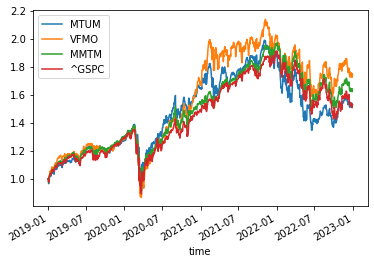
Momentum is a very interesting factor. It is very well documented and its performance is often regarded as a strong one, as with long-term trends it tends to outperform the index. If we look at the above chart, it is clear how all the funds outperformed during the period 2020-07 to 2022-01, and some of them even afterwards.

The rationale is relatively simple: as far as a stock is underperforming or overperforming, it will continue to do so. And in long-term trends, this happens, especially with low volatility.

An increase in volatility can, however, affect performance, and we can clearly observe this phenomenon after 2022: outperforming stocks might underperform in the upcoming month, then come back as winners, and momentum would lag behind them, tending to buy underperformers and sell overperformers.

Value

Value is likely the most interesting chart you will see today. What happened to value stocks?

First, we need to keep in mind that this group is usually opposed to growth stocks, which means companies that tend to invest much of their income to develop their business. Growth stocks tend to overperform in the long run, as they need to reach their full potential, but they also bring more risk. Value stocks are instead much more stable from a business perspective, but also undervalued, which means they might still overperform. Fama and French define the reason behind the existence of a value factor (and they found that low price-to-book ratio was the most predictive definition of it) in the following way:

The cross-section of book-to-market ratios might result from market overreaction to the relative prospects of firms. If overreaction tends to be corrected, BE/ME will predict the cross-section of stock returns.

This means that value itself performs well as far as markets look at financials. And from one point of view this is definitely important, but it is evident that there are many additional factors to consider.

Now, there is a consensus view that Value outperformed other factors in 2022. And it is not completely true, if we look at the figures in our Table 1: for example, the Dividend factor outperformed consistently (just look at tickers HDV, SDY and VYM, the best in terms of 2022 return).

So, what is the actual value behind Value? Probably not much from this perspective. We can consider value as a defensive factor: when bear markets happen, the price might fall much more than the actual valuation of stocks. Additionally, this factor normally exposes the portfolio to financials, utilities and cyclicals, which act as a defense from inflation and rising interest rates. Generally speaking, this factor tends to reward investors who are not scared by low prices and actually look at the underlying value of companies. But please, do not confuse the Value factor with Value Investing (Warren Buffett): they are completely different styles. The former tends to invest in companies which are undervalued according to some financial ratio, or a collection of those; the latter is a more specific style, which tends to make the business much more profitable, healthy and stable over the long term. And the latter usually does not diversify much.

Low Volatility

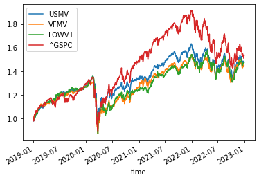
I bet this is another chart you will not forget.

Low volatility tends to outperform… during high volatility times! Does it sound counterintuitive? We can actually see how initially we have a very smooth bullish run (from 2020 to 2022 approximately), but afterwards (from 2022 on) we see a series of ups and downs, which we can identify as a very volatile time in the market. And in this time, the gap between the red line (S&P 500) and the others (low-volatility strategies) reduces dramatically. And this actually makes perfect sense: when volatility is high, normally there is a bear market. In this situation, the low-volatility premium increases, because stocks which move less will be left behind during long-term runs, but will also protect your portfolio when the more volatile businesses will suffer. So we expect this to actually behave defensively, and it is not a big surprise to see such performance.

However, let us focus on the performance in 2022 (Table 1). The tickers we need to look at are USMV (-8.87%), VFMV (-5.37%) and LOWV.L (-4.48%). They all still lost a considerable amount of money during the year (although much less than the S&P 500).

Why is this the case? Apart from the already-mentioned differences in implementation, we must keep in mind that investing in equity factors is not uncorrelated to the equity market. On the contrary, if we invested only in equity factors, we would not diversify our portfolio enough. But still, an overperformance relative to the S&P 500 of approximately +10% (USMV) or +15% (for the other two) is a very good achievement. So we can conclude that the intended behavior as a hedge is also benefiting our portfolio in practice.

Quality

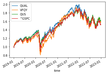
Quality is another factor often marketed as a diversifier/defensive hedge. During my time working for a defensive hedge fund, we had plenty of discussions with issuers of strategies such as hedges. But is it true that we can protect ourselves by investing in Quality?

Well, the answer is in the chart. If we look at the performance during the Covid period, not really. Although we see Quality as one of the overall best-performing factors, this is likely due to the long-term bullish runs (and as we see, the chart highlights some overperformance in the periods 2019-2020 before the Covid-19 pandemic and 2021, with the exception of the Vanguard ETF in orange), but it does not really protect your portfolio in market crashes. Maybe just slightly.

The iShares QUAL performance was the only one worse than the S&P 500 in 2022, for example. Generally speaking, Quality is indeed better than the index, but we must consider it an improvement, rather than a diversifier/hedge.

Dividend

Finally, another factor that works as a hedge!

It might seem crazy to be happy about such an underperforming investment right? But there is a but: the dividend factor is definitely going to give you some cash flows by definition, especially when we consider inflationary times!

Some studies show how dividends benefit investors during inflationary times, and this is relatively logical: while fixed-income securities have by definition a fixed rate, and thus they have additional risk when inflation comes up, for stocks, their dividends are not fixed, and as such, they can be increased by companies to attract investors. And inflation is definitely one of the factors contributing to increasing yields.

Moreover, dividends mean higher (total) returns and, as such, lower volatility.

Is factor investing scientific?

Recent publications suggest that factor investing does not imply scientific findings. This is a key observation that even Fama and French included in their 1992 paper:

Our main result is that two easily measured variables, size and book-to-market equity, seem to describe the cross-section of average stock returns. Prescriptions for using this evidence depend on (a) whether it will persist, and (b) whether it results from rational or irrational asset-pricing.

Factor investing is indeed a subset of systematic investments that comes from empirical evidence: as such, there is no theory or market inefficiency, but rather a very risky ex-post explanation (storytelling is often seen as one of the deadly sins of investing). And many companies offer additional factors, or tend to market their findings as innovations, while they likely just divided the universe of companies in a different way from before.

But we must also distinguish between soft sciences and hard sciences. As a soft science, finance will never be as causal as chemistry, biology and similar disciplines. Thus, it is also true that findings from empirical experiments are still useful and valid to the investing audience.

So, what should we do? We need to use them carefully, of course, like everything in investment. The first problem is factor timing: can we make some rotation to benefit from the more defensive factors (Dividend, Low Volatility, Value) while still being exposed to the most rewarding (Momentum, Quality)?

Some companies offer multi-factor strategies, with some weighting/rebalancing/allocation schemes that should benefit investors (net of all costs, of course). However, each of them might include some factors and exclude others, even just on a purely discretionary basis (if not for rebate interest in some ETF providers, but that’s another story…).

In this final exercise, I would like to show the performance of two simple strategies, an equally weighted portfolio and one with weights based on the characteristics of each factor (defensive or aggressive).

3) Portfolio Construction: Hypothetical Examples

Multi-factor portfolios

The simplest thing we can think of is: equal weights to every factor. Of course, please bear with me as this is not extremely scientific: we are just trying to make sense of the factor decomposition in equity returns in a very quick way. And of course, we have some look-ahead bias as we know how factors will perform (although their behavior is well known already from before 2019, where our study begins).

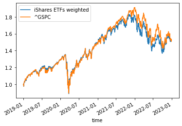
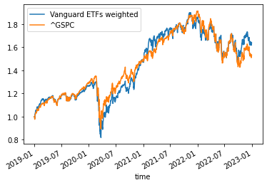
If we plot the equally weighted series vs the S&P 500, by distinguishing between providers, we can observe the following three charts:

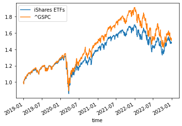
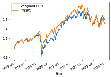
One of the most famous and successful ETF issuers, iShares, seems to considerably underperform its peers from this perspective.

Now, what would happen if we instead assigned the following weights to each factor:
35% each to Momentum and Quality (aggressive factors), for a total of 70%, and
10% each to Dividend, Value and Low Volatility (defensive factors), for a total of 10%.

Again, we will just distinguish between providers and plot the final returns here.

It doesn’t seem like a lot, but it is such an improvement instead! Let’s have a look at their summary performance in Table 2:

It is clear that a weighting scheme that considers the profile of the factors will only benefit the overall portfolio performance. For comparison, the S&P 500 delivers a 53.16% return (11.25% annualized). Only the iShares ETF fails to outperform it.

The cost is of course very small as we invest only at the beginning of our testing period (2018-12-31). And of course it might be worth testing something more sophisticated, like rebalancing signals (some papers attempt using sophisticated tools like nowcasting).

ETF comparison

And what should we prefer in terms of an ETF issuer for every factor? Of course, we will not analyze only returns, as this would be a horrible decision. Generally speaking, there is no single performance indicator that would work alone.

But with a collection of indicators we might get a sense of how the funds differ between each other and what we might prefer, on the basis of risk aversion and maybe correlation to the rest of our portfolio. For now, we will only consider a general and simple profile of the funds.

Figures are annualized to compare them on a yearly basis. We will focus our analysis on a few basic indicators:

1. Annualized return. The return achieved by year, keeping in mind compounding.
2. Annualized volatility. The volatility of the achieved return on an annual basis, which means how ‘different’ (on the upside or downside) the return might be on an annual basis compared with the average return.
3. Sharpe Ratio. The ratio between return and volatility (both annualized, in this case). It defines the general risk-reward profile: for every unit of risk (1% in volatility), we will be rewarded according to the Sharpe Ratio. The higher it is, the higher our return on the basis of the risk assumed. We assume a risk-free rate of 0 for simplicity.
4. Beta to S&P 500. This expresses the systemic risk of an investment, which means the expected percentage change for a 1% change in the index.
   Expense ratio. This reflects how much a fund pays for its expenses, including portfolio management, marketing, custody etc.

Momentum

While momentum is by itself a relatively clear factor, we can appreciate the differences between the three funds, suggesting that implementation and costs do matter.

In terms of return, Vanguard’s VFMO shows higher figures. However, if we look at the Sharpe Ratio, this difference is cleared out when compared against MMTM: this expresses the better risk-management profile of the latter, as the reward per unit of risk is higher.

Beta is also very important, as profits and losses due to systemic risk might be amplified by the funds, depending on their strategy and setup: fortunately this is not the case for momentum as a whole, but MMTM does a better job of diversifying risk and it also keeps the general volatility of the fund lower.

Finally, when comparing costs, the difference is not extreme, but MMTM also offers a cheaper profile in this sense, meaning that investors will be charged less for operational expenses.

Value

Value investing can differ quite significantly between funds, as we already stated. And indeed, what we see is that the three funds really differ even just from a return perspective.

In this case, Vanguard’s fund seems to offer more upside potential. However, we must keep in mind that volatility is much higher. This results in a lower Sharpe Ratio than SPYV: it appears that the latter performs better in terms of return per unit of risk.

Volatility is not telling us everything from a risk perspective. In this sense, we should also look at systemic risk, as it would advise us on how sensitive the funds are to the moves in the market, using Beta. And in this case, Beta is higher than 1 for two of the funds (1.01 for VLUE and 1.10 for VFVA), suggesting that the funds are generally aggressive (for example, for every +1% move of S&P 500, VFVA earns +1.10%; however, for every -1% move, it loses -1.10%); the exception here is provided by SPYV, which moves 10bps less. This is also the message we can get from looking at volatilities: lower volatility means a more moderate profile in terms of return variation, both on the upside and downside.

Finally, if we look at the expense ratio, it appears that SPYV also detracts considerably less from performance for its investors in terms of costs.

Low Volatility

While being also relatively simple, we have already appreciated the different profiles of the low volatility factor.

When annualizing, the figures seem much closer than initially. However, the clear advantage is that LOWV.L performs with a much more defensive approach than the other two, showing how risk management is, again, a priority for State Street.

In terms of the Sharpe Ratio, the three funds are similar, but we appreciate the lower Beta and higher return of LOWV.L. This time, the expense ratio sounds a bit high compared to the other two (more than double!), and we might want to consider if this is worth the investment, or if we would rather invest in a more aggressive fund like iShares’ USMV which keeps costs lower.

Quality

In this case, the difference in the above chart was not that remarkable. And in terms of performance, this is reflected in the below table.

Again, on the risk side, State Street’s QUS seems the best performer, as well as from a Sharpe Ratio perspective. However, the cost is higher than VFQY, suggesting that, after fees, it might be less convenient than it seems.

Dividend

We conclude our factor analysis with the dividend factor.

It is striking how the iShares and Vanguard funds have lower fees, while State Street keeps them much higher. Additionally, in this case, it seems like SDY is not the best in terms of Beta and volatility as well (and, additionally, its Sharpe Ratio is lower than VYM). So the most reasonable choice would probably be VYM.

4) Outlook for 2023

With a stagnant economy, high inflation and low real income, the current environment does not favor equities. The recent bank turmoil, and the uncertainty about the job market, growth forecasts and interest rates are also weighing down on the performance of equities. Amid this gloomy outlook, factor investing – in particular based on value, low volatility and dividend – is believed to be capable of boosting investors’ portfolios significantly.

From the performance, it seems clear that, if 2023 turns out to be like 2022 (and at the moment there are plenty of risky events, like banks, inflation, geopolitical tensions, layoffs, etc), these factors could outperform the broader index significantly. And if we want to still keep some upside potential, in case the bad forecasts do not happen, we should still stick to a variety of factors, for example by keeping some exposure to momentum. Factor investing, and in particular the different risk profile of factors, can generally help in diversifying equity portfolios.

However, we must keep in mind that there are other asset classes which can outperform equities, and offer diversification benefits. This specific analysis only refers to factor investing relative to equities, and a balanced portfolio should never concentrate on a single asset class.

From what we learned, we could hypothesize a few equity portfolios which would make sense for three possible views: A) US Equities will perform very well in 2023; B) US Equities could perform well, but we will protect our portfolio enough to outperform the benchmark; C) US Equities will have another horrible year. Please note that this is not financial advice, but rather an exercise to see how to implement different views on the market. Please also note that there’s no consensus view as to what constitutes an “aggressive”, “balanced” or “defensive” portfolio – I am only constructing the portfolios below as a thought experiment.

Option A: Aggressive Portfolio - Equities will perform very well
90% Aggressive -> 60% Momentum, 30% Quality
10% Defensive -> 10% Dividend

In case of a bullish run, volatility will (likely) be low, and we want some cash flows as inflation is anyway going to be relatively high throughout the year. Thus, the defensive part of the portfolio (which is a minimal one in this case as we believe we do not need to protect us much) will be composed of Dividends only. The rest is aggressive, and Quality is an improved version of the benchmark, as we have seen, while Momentum would be the outperformer in the aggressive scenario.

Option B: Balanced Portfolio - Uncertainty ahead
70% Aggressive -> 40% Quality, 30% Momentum
30% Defensive -> 10% Dividend, 10% Low Volatility, 10% Value

This portfolio would be open to the upside, but still with some downside protection. However, we prefer to remain cautious and be closer to the index with Quality rather than Momentum. On the defensive side, Dividend is still preferred, but we add Low Volatility to diversify. Value is a factor that outperformed recently, and it could continue to do so, given the global layoffs in tech (usually associated with growth) and high interest rate environment.

Option C: Defensive Portfolio - Protecting against the selloff
50% Aggressive -> 40% Quality, 10% Momentum
50% Defensive -> 20% Dividend, 20% Low Volatility, 10% Value

In case of a selloff, our aggressive portfolio should definitely reduce its Momentum exposure. Quality is the best choice for the aggressive part of our portfolio. On the defensive side, we keep some exposure to Value as it might get a year similar to the last one, but we prefer to keep equal portions of Dividend and Low Volatility, which, from my perspective, better protect during hard times in equities.

Conclusion

Factor investing is a well established concept in the financial industry. As a whole, it intends to dissect returns into explainable factors. It has some favorable features, such as:

1. Explainability: we can explain factors in a very straightforward fashion;
2. Supporting literature: many have researched and deployed these strategies into production or academic papers;
3. Diversification benefits: some of these factors improve the (equity) portfolio by lowering risk;

But it also suffers from some pitfalls, namely:

1. Alpha decay: many have used these kind of strategies, and as such, it is not really useful to add alpha to your portfolio;
2. Too many choices: there are plenty of factors, and investors might find it difficult to understand which factors to invest in;
3. Unclear methodologies: it can happen that funds implement very generic strategies (e.g. for Quality: ‘selecting high-quality businesses from the universe’ might be expressed in so many ways…) and eventually investors are exposed to different factors than those they initially expected.

Considering the benefits of it, we can conclude it is certainly a useful strategy that will improve the equity profile of a portfolio. It is, however, problematic to discern between consistent and less consistent factors, especially in some cases, such as Value or Size, which, although offering the mentioned benefits, have deteriorated performance as a whole in recent years.

My expectation in the future is that we will slowly transition away from this kind of strategy. It is a very crowded space, and it is also not adding to performance as many might think.

Some suggest that factor investing is still at the prototyping stage in other asset classes, such as fixed income or forex; and indeed, factors in these asset classes are much less known, and often have a very different profile from their equity counterparts. This is definitely a direction for present and future quant research. However, it is now time to offer something more sophisticated and scientific to investors.

Finally, here’s my monthly watchlist of portfolio strategies, including those mentioned above (for factors, I used State Street’s ETFs for all factors):